
Understanding Diffusion Models by Coding
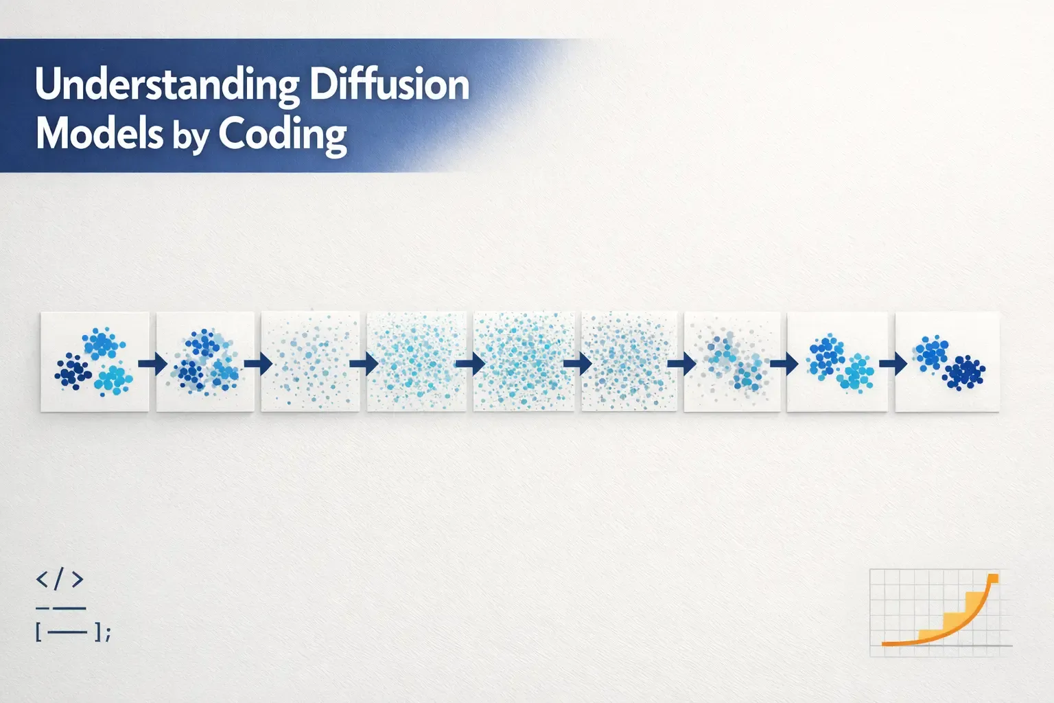
Minimal example for diffusion models with code and equations
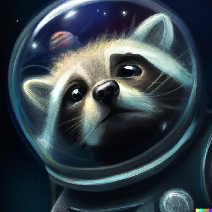
Diffusion models have recently gained popularity due to their success at generating photorealistic images with/ without text prompt. They are at the core of models like Dall-e or imagen.
The goal of this post is to explain the forward and reverse flow of a diffusion model with code and equations from the paper so as to allow users to better understand the overall process.
For people who’d prefer directly diving into the code, visit the repo https://github.com/InFoCusp/diffusion_models or directly the colab: https://colab.research.google.com/github/InFoCusp/diffusion_models/blob/main/Diffusion_models.ipynb
Diffusion models are a family of models that have shown amazing capability of generating photorealistic images with/ without text prompt. They have two flows as shown in the figure below -
- Deterministic forward flow (from image to noise) and
- Generative reverse flow (recreating image from noise).
They get their name from the forward flow where they follow a markov chain of diffusion steps, each of which adds a small amount of random noise to the data. Then they learn the model to reverse the diffusion process and construct desired data samples from noise.
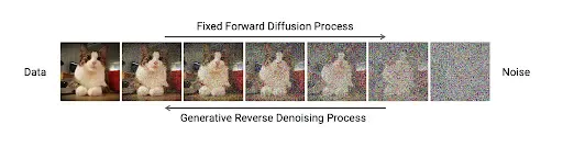
Forward and reverse flow. Source: https://developer.nvidia.com/blog/improving-diffusion-models-as-an-alternative-to-gans-part-1/
Since they map noise to data, these models can be said to be capable of learning the distributions that generate data of any particular domain. Let’s step into step -1, generating image like data but with less dimensions for the model to learn from.
Data Distribution
Images can be thought of as points sampled from height×width dimensional space.
Consider an image of dimension height×width. Then the total number of pixels are height×width. Each pixel has a value ranging from 0 to 255. Now, consider a vector space, where we flatten this image and represent the intensity of each pixel along one dimension of the vector space. For example, an image with height=2 and width=3 (2px x 3px image) becomes a single vector of length 6 where each component of this vector will have a value between 0 to 255.
So, in this image vector space, there are small clusters of valid (photorealistic) images sparsely distributed over the space. Rest of the vector space is made up of invalid (not real looking) images.
For the example in this notebook, we consider a hypothetical simplified version of the above representation. We consider images made of just 2 pixels, each of which can have values between [-5, 5]. This is to allow visualization of each dimension of the data as it moves through the forward and reverse process (and additionally faster training 😅).
The same code can be extended to the original image dimensions with just updated data dimensions.
# Generate original points which are around [0.5, 0.5] in all quadrants and
# 4 corners ([0,1], [1,0], [0,-1], [-1, 0])
# Some region around these points indicates valid images region (true data distribution)
num_samples_per_center = 1000
stddev = 0.1
mean = 0
centers = tf.constant([[0,1], [1,0], [0,-1], [-1, 0],
[0.5, 0.5], [0.5, -0.5], [-0.5, -0.5],
[-0.5,0.5]]) * 4
all_data = []
# Data for all clusters
for idx in range(centers.shape[0]):
center_data = tf.random.normal(shape=(num_samples_per_center, 2), stddev=stddev, mean=mean + centers[idx,:], dtype=tf.float32)
all_data.append(center_data)
# X,_ = sklearn.datasets.make_moons(8000)
train_data_tf = tf.concat(all_data, axis=0)
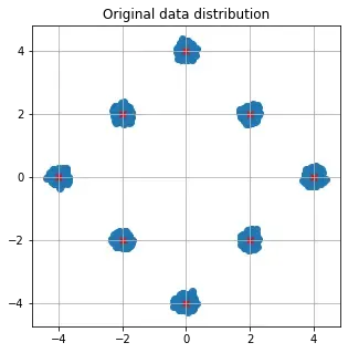
print(f'{train_data_tf.shape[0]} samples of {train_data_tf.shape[1]} dimensions in training data')The x’s in the plot below can be thought of as valid images in 2d space with the rest of the white region representing the rest of the invalid images. The blue clusters around the x’s are also valid images (corresponding to minor pixel perturbations in original images).
Beta Schedule
Now that we have the original (non noisy) data, let’s start with the actual diffusion implementation. The first thing is to add noise to the input images following a fixed variance schedule (also known as beta schedule). The original paper uses a linear schedule. And 1000 timesteps to move forward and back. We use smaller number of timesteps (250) as the data is simpler in our case.
num_diffusion_timesteps=250
beta_start=0.0001
beta_end=0.02
schedule_type='linear'
def get_beta_schedule(schedule_type, beta_start, beta_end, num_diffusion_timesteps):
if schedule_type == 'quadratic':
betas = np.linspace(beta_start ** 0.5, beta_end ** 0.5, num_diffusion_timesteps, dtype=np.float32) ** 2
elif schedule_type == 'linear':
betas = np.linspace(beta_start, beta_end, num_diffusion_timesteps, dtype=np.float32)
return betas
betas_linear = get_beta_schedule('linear', beta_start, beta_end, num_diffusion_timesteps)
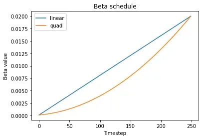
betas_quad = get_beta_schedule('quadratic', beta_start, beta_end, num_diffusion_timesteps)Visualize beta schedules
The below plot shows that the variance of noise is low at the start and increases as we move forward in time.
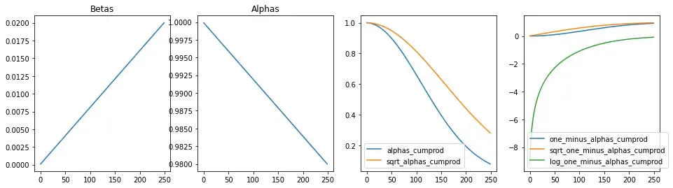
Beta derivatives
Next, let’s compute all the derivatives from beta that are used repeatedly in the forward and reverse process of diffusion. Since the variance schedule ( βt ) is fixed, the derivatives of βt are also fixed. We precompute these to save time/ compute.
We’ll see the use cases of these variables in the respective sections below.
class BetaDerivatives():
  def __init__(self, betas, dtype=tf.float32):
    """Take in betas and pre-compute the dependent values to use in forward/ backward pass.

    Values are precomputed for all timesteps so that they can be used as and
    when required.
    """
    self.np_betas = betas
    timesteps, = betas.shape
    self.num_timesteps = int(timesteps)

    self.betas = tf.constant(betas, dtype=dtype)
    self.alphas = tf.subtract(1., betas)
    self.alphas_cumprod = tf.math.cumprod(self.alphas, axis=0)
    self.alphas_cumprod_prev = tf.concat([tf.constant([1.0]), self.alphas_cumprod[:-1]], axis=0)

    # calculations required for diffusion q(x_t | x_{t-1}) and others
    self.sqrt_alphas_cumprod = tf.math.sqrt(self.alphas_cumprod)
    self.sqrt_one_minus_alphas_cumprod = tf.math.sqrt(1. - self.alphas_cumprod)
    self.log_one_minus_alphas_cumprod = tf.math.log(1. - self.alphas_cumprod)


  def _gather(self, a, t):
    """
    Utility function to extract some coefficients at specified timesteps,
    then reshape to [batch_size, 1] for broadcasting.
    """
    return tf.reshape(tf.gather(a, t), [-1, 1])
Visualize beta derivatives over time
Forward pass of diffusion model
In the forward pass, the diffused input at timestep t can be computed directly using the closed form equation (For derivation of how we arrive at this, refer to the paper: https://arxiv.org/pdf/2006.11239.pdf.
$$ q\left(x_t \mid x_0\right)=N\left(\sqrt{\bar{\alpha}_t} x_o, 1-\overline{\alpha_t} I\right) $$
This is done in the q_sample function below.
class DiffusionForward(BetaDerivatives):
  """
  Forward pass of the diffusion model.
  """

  def __init__(self, betas):
    super().__init__(betas)


  def q_sample(self, x_start, t, noise=None):
    """
    Forward pass - sample of diffused data at time t.
    """
    if noise is None:
      noise = tf.random.normal(shape=x_start.shape)
    p1 = self._gather(self.sqrt_alphas_cumprod, t) * x_start
    p2 = self._gather(self.sqrt_one_minus_alphas_cumprod, t) * noise
    return (p1 + p2)

diff_forward = DiffusionForward(betas_linear)
Visualize the forward diffusion of the entire data over time
We start with original data distribution and move it through the forward diffusion process 10 steps at a time. We can see that the original data distribution information is lost till it resembles gaussian after num_diffusion_steps.
Also, the slow perturbations at the start and large ones towards the end as per the beta schedule are evident from the video.
Model building
With the data taken care of, let’s build a model that can fit the data. We use a DNN with few layers since we’re just using data with 2 features that we wish to reconstruct. Would be replaced with unet with similar loss function for the case of image data.
The model takes in 2 inputs:
- Timestep embedding of t
- xt
And predicts
- the noise n that lead from x0 to xt.
Let’s first code the timestep embedding:
# We create a 128 dimensional embedding for the timestep input to the model.
# Fixed embeddings similar to positional embeddings in transformer are used -
# could be replaced by trainable embeddings later


def get_timestep_embedding(timesteps, embedding_dim: int):
  half_dim = embedding_dim // 2
  emb = tf.math.log(10000.0) / (half_dim - 1)
  emb = tf.exp(tf.range(half_dim, dtype=tf.float32) * -emb)
  emb = tf.cast(timesteps, dtype=tf.float32)[:, None] * emb[None, :]
  emb = tf.concat([tf.sin(emb), tf.cos(emb)], axis=1)
  if embedding_dim % 2 == 1:  # zero pad
    # emb = tf.concat([emb, tf.zeros([num_embeddings, 1])], axis=1)
    emb = tf.pad(emb, [[0, 0], [0, 1]])
  return emb


temb = get_timestep_embedding(tf.constant([2,3]),128)
print(temb.shape)
And now the actual model which is just a DNN for 2d data to its reconstruction
# Actual model that takes in x_t and t and outputs n_{t-1}
# Experiments showed that prediction of n_{t-1} worked better compared to
# prediction of x_{t-1}


def build_model():
  input_x = tf.keras.layers.Input(train_data_tf.shape[1])
  temb = tf.keras.layers.Input(128)


  # temb = tf.keras.layers.Reshape((128,))(tf.keras.layers.Embedding(1000, 128)(input_t))
  d1 = tf.keras.layers.Dense(128)(input_x)
  merge = tf.keras.layers.Concatenate()((temb, d1))
  d2 = tf.keras.layers.Dense(128, 'relu')(merge)
  d2 = tf.keras.layers.Dense(64, 'relu')(d2)
  d2 = tf.keras.layers.Dense(32, 'relu')(d2)
  d3 = tf.keras.layers.Dense(16, 'relu')(d2)
  d4 = tf.keras.layers.Dense(2)(d3)
  model = tf.keras.Model([input_x, temb], d4)
  return model


model = build_model()
print(model.summary())
model.compile(loss='mse', optimizer='adam')
Data generation for diffusion model
Next, let’s generate the data for the model to train. We generate xt given the input x0 using the deterministic forward process equation described above. This xt and timestep embedding of t are input to the model that is tasked with predicting the noise n . t is picked uniformly between [0, num_diffusion_timesteps]
shuffle_buffer_size = 1000
batch_size = 32


def data_generator_forward(x, gdb):
  tstep = tf.random.uniform(shape=(tf.shape(x)[0],), minval=0, maxval=num_diffusion_timesteps, dtype=tf.int32)
  noise = tf.random.normal(shape = tf.shape(x), dtype=x.dtype)
  noisy_out = gdb.q_sample(x, tstep, noise)
  return ((noisy_out, get_timestep_embedding(tstep, 128)), noise)


# Model takes in noisy output and timestep embedding and predicts noise
dataset = tf.data.Dataset.from_tensor_slices((train_data_tf)).shuffle(shuffle_buffer_size).batch(batch_size)
dataset = dataset.map(functools.partial(data_generator_forward, gdb=diff_forward))
Let’s test the data generator
# Let's test the data generator
(xx,tt),yy = next(iter(dataset))
print(xx.shape, tt.shape, yy.shape)

### (32, 2) (32, 128) (32, 2)
After a training for 200 epochs that takes roughly 2-3 minutes, we get the below results.
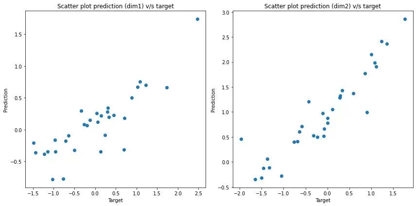
Scatter plots of reconstructed values v/s target
When there is a perfect match between the prediction and target, the scatter plot would be a line along y=x (45 degrees in the first quadrant). We observe similar behaviour in the plot below indicating that the model has is able to predict the target decently.
Reverse process of diffusion
The model provides a decent estimate of the noise given the data and t. Now comes the tricky part: given the data at timestep t$x_t$, and the noise estimate from the model, reconstructing original data distribution.
There are 4 parts in the reverse process:
-
Pass $x_t$ and t (converted to time embedding) into the model that predicts the noise $\epsilon$
-
Using the noise estimate $\epsilon$ and $x_t$, compute $x_0$ using equation:
$$ \frac{1}{\sqrt{\bar{\alpha}_t}} x_t-\left(\sqrt{\frac{1}{\bar{\alpha}_t}-1}\right) \epsilon $$
- Compute mean and variance using the equations:
$$ \tilde{\mu}\left(x_t, x_0\right)=\frac{\sqrt{\bar{\alpha}_{t-1}} \beta_t}{1-\bar{\alpha}_t} x_0+\frac{\sqrt{\bar{\alpha}t}\left(1-\bar{\alpha}{t-1}\right)}{1-\bar{\alpha}_t} x_t $$
and variance $\tilde{\beta}t=\frac{\left(1-\bar{\alpha}{t-1}\right)}{1-\bar{\alpha}_t} \beta_t$
- Sample using this mean and variance $q\left(x_{t-1} \mid x_t, x_0\right)=N\left(x_{t-1} ; \tilde{\mu}\left(x_t, x_0\right), \tilde{\beta}_t I\right)$
class DiffusionReconstruct(BetaDerivatives):

  def __init__(self, betas):
    super().__init__(betas)

    self.sqrt_recip_alphas_cumprod = tf.math.sqrt(1. / self.alphas_cumprod)
    self.sqrt_recipm1_alphas_cumprod = tf.math.sqrt(1. / self.alphas_cumprod - 1)

    # calculations required for posterior q(x_{t-1} | x_t, x_0)
    # Variance choice corresponds to 2nd choice mentioned in the paper
    self.posterior_variance = self.betas * (1. - self.alphas_cumprod_prev) / (1. - self.alphas_cumprod)


    # below: log calculation clipped because the posterior variance is 0 at the beginning of the diffusion chain
    self.posterior_log_variance_clipped = tf.constant(np.log(np.maximum(self.posterior_variance, 1e-20)))
    self.posterior_mean_coef1 = self.betas * tf.math.sqrt(self.alphas_cumprod_prev) / (1. - self.alphas_cumprod)
    self.posterior_mean_coef2 = (1. - self.alphas_cumprod_prev) * tf.math.sqrt(self.alphas) / (1. - self.alphas_cumprod)

  def predict_start_from_noise(self, x_t, t, noise):
    """
    Reconstruct x_0 using x_t, t and noise. Uses deterministic process
    """
    return (
        self._gather(self.sqrt_recip_alphas_cumprod, t) * x_t -
        self._gather(self.sqrt_recipm1_alphas_cumprod, t) * noise
    )


  def q_posterior(self, x_start, x_t, t):
    """
    Compute the mean and variance of the diffusion posterior q(x_{t-1} | x_t, x_0)
    """
    posterior_mean = (
        self._gather(self.posterior_mean_coef1, t) * x_start +
        self._gather(self.posterior_mean_coef2, t) * x_t
    )
    posterior_log_variance_clipped = self._gather(self.posterior_log_variance_clipped, t)
    return posterior_mean, posterior_log_variance_clipped


  def p_sample(self, model, x_t, t):
    """
    Sample from the model. This does 4 things
    * Predict the noise from the model using x_t and t
    * Create estimate of x_0 using x_t and noise (reconstruction)
    * Estimate of model mean and log_variance of x_{t-1} using x_0, x_t and t
    * Sample data (for x_{t-1}) using the mean and variance values
    """
    noise_pred = model((x_t, get_timestep_embedding(t, 128))) # Step 1
    x_recon = self.predict_start_from_noise(x_t, t=t, noise=noise_pred) # Step 2
    model_mean, model_log_variance = self.q_posterior(x_start=x_recon, x_t=x_t, t=t) # Step 3
    noise = noise_like(x_t.shape)
    nonzero_mask = tf.reshape(tf.cast(tf.greater(t, 0), tf.float32), (x_t.shape[0], 1))
    return model_mean + tf.exp(0.5 * model_log_variance) * noise * nonzero_mask # Step 4


  def p_sample_loop_trajectory(self, model, shape):
    """
    Generate the visualization of intermediate steps of the reverse of diffusion
    process.
    """
    times = tf.Variable([self.num_timesteps - 1], dtype=tf.int32)
    imgs = tf.Variable([noise_like(shape)])
    times, imgs = tf.while_loop(
      cond=lambda times_, _: tf.greater_equal(times_[-1], 0),
      body=lambda times_, imgs_: [
        tf.concat([times_, [times_[-1] - 1]], axis=0),
        tf.concat([imgs_, [self.p_sample(model=model,
                                         x_t=imgs_[-1],
                                         t=tf.fill([shape[0]], times_[-1]))]],
                  axis=0)
      ],
      loop_vars=[times, imgs],
      shape_invariants=[tf.TensorShape([None, 1]),
                        tf.TensorShape([None, *shape])],
      back_prop=False
    )
    return times, imgs
In the video explaining the reverse process: , we show the reconstruction process of the data from noise. We start with 1000 samples from std. normal distribution (gaussian noise) and iteratively move towards the original data distribution using the model trained above.
As you can see towards the end of the video, the noise maps back to the original data distribution.
Voila! We just showcased the diffusion model workflow with a minimal example that can train within minutes.
If you found the explanation/ code helpful please star/ share the repo: https://github.com/InFoCusp/diffusion_models
References:


